39 how to format data labels in excel charts
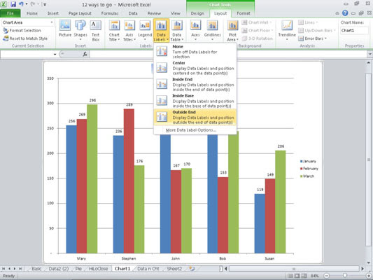
How to format bar charts in Excel - storytelling with data Click on any data label to highlight them all, then right-click and choose Format Data Labels: 4. In the Format Data Labels menu, select Label Options, and in the Label Positions section, choose Inside End. (While you're at it, in the Label Contains section, uncheck "Show Leader Lines." These are almost never necessary.) Pivot Chart Data Label Formatting Question - Microsoft Tech Community I format the data labels, for example make the text larger or turn it. Every time I refresh the data the data label formatting reverts to the default. I have gone to the Pivot Chart options and made sure the Preserve cell formatting option is checked. How to I get around this and preserve my data label formatting when the data is refreshed?
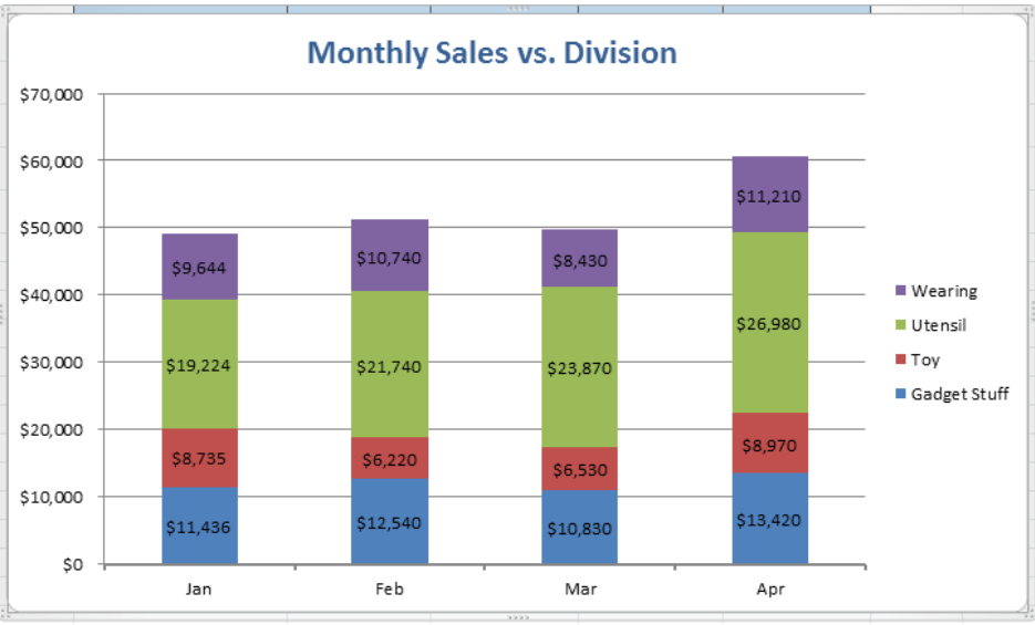
How can I get data labels to show for each column in a bar chart? Turn on 'Overflow text' under Data label' Format tab. Also, you can adjust the position of the Data Label by switching to 'Outside End' or 'Inside Center' so that your Data Label gets displayed properly. If this post helps, then mark it as 'Accept as Solution ' so that it could help others. Regards, Sanket Bhagwat.
How to format data labels in excel charts
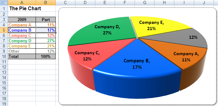
Excel Pivot Table Filter and Label Formatting - Microsoft Tech Community Excel 2016 Images of 2 separate workbooks, each with a data table, pivot table and pivot chart, the one on the right created by copy & paste of the one on the left. The one on the right changed: X axis labels on the pivot chart don't have the multi-level option. Also, unlike the original on the... Pie of Pie Chart in Excel - Inserting, Customizing, Formatting To order to format the data labels, right-click on any one of them and select format data labels from the shortcut menu. This is going to open a Format Data Labels pane at the right of excel. Mark the percentage, category name, and legend key. Select the position of data labels at Outside End. How to: Display and Format Data Labels - DevExpress To apply a number format to data labels, utilize the DataLabelBase.NumberFormat property, which provides access to the NumberFormatOptions object containing format options for displaying numbers in different chart elements. Next, assign the corresponding number format code to the NumberFormatOptions.FormatCode property.
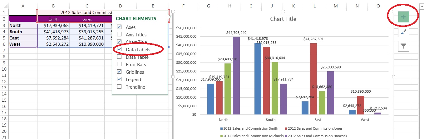
How to format data labels in excel charts. How can I format individual data points in Google Sheets charts? Note, custom formatting can be applied to individual data points by right clicking them from within the chart: How to add labels to specific data points only? In the example below, I used data labels to clearly indicate the sales figures for the end of each day, during a 3-day digital flash sale, which helped the client easily see their ... Custom Chart Data Labels In Excel With Formulas Follow the steps below to create the custom data labels. Select the chart label you want to change. In the formula-bar hit = (equals), select the cell reference containing your chart label's data. In this case, the first label is in cell E2. Finally, repeat for all your chart laebls. How to Create Bar of Pie Chart in Excel - Computing.NET Step 1: Highlight the entire range. Step 2: Click on the Insert tab, Step 3: Navigate to the Chart grouping and click on the Insert Pie or Doughnut Chart icon. A drop-down box of Pie options is displayed. Step 4: Select the Bar of a Pie icon under the 2D pie category. This creates the combination as shown below. How to Add Labels to Scatterplot Points in Excel - Statology Step 3: Add Labels to Points. Next, click anywhere on the chart until a green plus (+) sign appears in the top right corner. Then click Data Labels, then click More Options…. In the Format Data Labels window that appears on the right of the screen, uncheck the box next to Y Value and check the box next to Value From Cells.
How to Create a Run Chart in Excel (2021 Guide) | 2 Free Templates Step 2. Build a Line Chart. Now that you have recorded the median values, you have all the data you need to build out your run chart. Highlight any cell in the expanded data table ( A1:C14 ). Go to the Insert tab. Click " Insert Line or Area Chart .". Choose " Line .". Chart.ApplyDataLabels method (Excel) | Microsoft Docs For the Chart and Series objects, True if the series has leader lines. Pass a Boolean value to enable or disable the series name for the data label. Pass a Boolean value to enable or disable the category name for the data label. Pass a Boolean value to enable or disable the value for the data label. How to Format Excel Charts - Naukri Learning To format data labels or a trend line label, double-click the element On the Number tab, select the options that you want Change Axis Labels in a Chart A label identifies each category on the horizontal axis. You can change the intervals at which these labels and minor tick marks appear. How to Find, Highlight, and Label a Data Point in Excel Scatter Plot? By default, the data labels are the y-coordinates. Step 3: Right-click on any of the data labels. A drop-down appears. Click on the Format Data Labels… option. Step 4: Format Data Labels dialogue box appears. Under the Label Options, check the box Value from Cells . Step 5: Data Label Range dialogue-box appears.
How to Make a Pie Chart in Excel - WinBuzzer Click on your pie chart in Excel and choose a style from the "Chart Design" tab. You'll find various styles above the "Chart Styles" heading which will give your chart a fresh look ... Formatting Long Labels in Excel - PolicyViz Copy your graph Open PowerPoint and Paste the graph. Don't worry about the slide size or anything, just paste it in. Select the axis you want to format and select the Format option in the Paragraph menu. In the ensuing menu, select the Right option in the Alignment drop-down menu. Change the format of data labels in a chart - Microsoft Support DataLabels object (Excel) | Microsoft Docs The following example sets the number format for data labels on series one on chart sheet one. With Charts(1).SeriesCollection(1) .HasDataLabels = True .DataLabels.NumberFormat = "##.##" End With Use DataLabels (index), where index is the data-label index number, to return a single DataLabel object. The following example sets the number format ...
Excel Charts: Creating Custom Data Labels - YouTube
How To Add Data Labels In Excel Guide 2022 - IND4 Blog Take a good look at your excel worksheet. Click add data label, then click add data callout. Source: hima4.cdtla.org. To format data labels, select your chart, and then in the chart design tab, click add chart element > data labels > more data label options. The result is that your data label will appear in a graphical.
How to Add Data Labels in Excel - Excelchat | Excelchat
How to Change the Y Axis in Excel - Alphr Click on the "Chart Tools" and then "Design" and "Format" tabs. When you open the "Format" tab, click on the "Format Selection" and click on the axis you want to change.

Enable or Disable Excel Data Labels at the click of a button - How To - PakAccountants.com
How to Create and Customize a Treemap Chart in Microsoft Excel Either right-click the chart and pick "Format Chart Area" or double-click the chart to open the sidebar. On Windows, you'll see two handy buttons on the right of your chart when you select it. With these, you can add, remove, and reposition Chart Elements. And you can pick a style or color scheme with the Chart Styles button.

Excel 3-D Pie charts - Microsoft Excel 2016
Excel Waterfall Chart: How to Create One That Doesn't Suck Click inside the data table, go to " Insert " tab and click " Insert Waterfall Chart " and then click on the chart. Voila: OK, technically this is a waterfall chart, but it's not exactly what we hoped for. In the legend we see Excel 2016 has 3 types of columns in a waterfall chart: Increase. Decrease.

Excel Course: Inserting Graphs
How to Create and Customize a Waterfall Chart in Microsoft Excel To fix this, double-click the chart to display the Format sidebar. Select the bar for the total by clicking it twice. Click the Series Options tab in the sidebar and expand Series Options if necessary. Check the box for "Set as Total." Then, do the same for the other total.

Surface Chart in Excel
Excel: How to Create a Bubble Chart with Labels - Statology Step 3: Add Labels. To add labels to the bubble chart, click anywhere on the chart and then click the green plus "+" sign in the top right corner. Then click the arrow next to Data Labels and then click More Options in the dropdown menu: In the panel that appears on the right side of the screen, check the box next to Value From Cells within ...

How to Create Multi-Category Chart in Excel - Excel Board
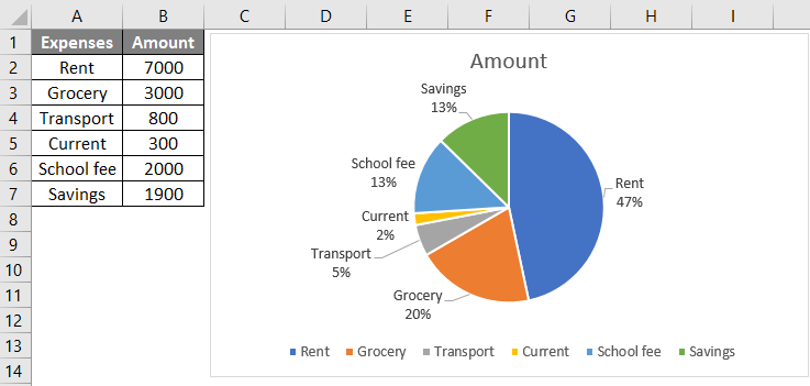
Pie Chart in Excel - Inserting, Formatting, Filters, Data Labels Right click on the Data Labels on the chart. Click on Format Data Labels option. Consequently, this will open up the Format Data Labels pane on the right of the excel worksheet. Mark the Category Name, Percentage and Legend Key. Also mark the labels position at Outside End. This is how the chark looks. Formatting the Chart Background, Chart Styles
Pie Chart Examples | Types of Pie Charts in Excel with Examples
How to Print Labels from Excel - Lifewire Select Mailings > Write & Insert Fields > Update Labels . Once you have the Excel spreadsheet and the Word document set up, you can merge the information and print your labels. Click Finish & Merge in the Finish group on the Mailings tab. Click Edit Individual Documents to preview how your printed labels will appear. Select All > OK .

Excel Chart Elements: Parts of Charts in Excel | ExcelDemy
excel - Formatting Data Labels on a Chart - Stack Overflow sub charttest () activesheet.chartobjects ("chart 6").activate z = 1 with activechart if .charttype = xlline then i = .seriescollection (1).points.count activechart.fullseriescollection (1).datalabels.select for pts = 1 to i activechart.fullseriescollection (1).points (pts).hasdatalabel = true ' make sure all points are visible data …
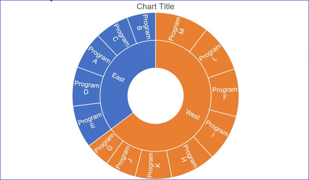
How to Make a Sunburst Chart - ExcelNotes
How to Show Percentages in Stacked Column Chart in Excel? Implementation: Follow the below steps to show percentages in stacked column chart In Excel: Step 2: Select the entire data table. Step 3: To create a column chart in excel for your data table. Go to "Insert" >> "Column or Bar Chart" >> Select Stacked Column Chart. Step 4: Add Data labels to the chart. Goto "Chart Design" >> "Add ...
Microsoft Tips with Temo!: How to Add Data Labels to an Excel 2010 Chart
How To Create Labels In Excel | RR BLog Source: labels-top.com. Right click the data series in the chart, and select add data labels > add data labels from the context menu to add data labels. Column names in your spreadsheet match the field names you want to insert in your labels. Source: . Click the expand selection icon to have the entire table.
Excel 3-D Pie Charts
How to: Display and Format Data Labels - DevExpress To apply a number format to data labels, utilize the DataLabelBase.NumberFormat property, which provides access to the NumberFormatOptions object containing format options for displaying numbers in different chart elements. Next, assign the corresponding number format code to the NumberFormatOptions.FormatCode property.
Data Driven Polar Charts for PowerPoint - SlideModel
Pie of Pie Chart in Excel - Inserting, Customizing, Formatting To order to format the data labels, right-click on any one of them and select format data labels from the shortcut menu. This is going to open a Format Data Labels pane at the right of excel. Mark the percentage, category name, and legend key. Select the position of data labels at Outside End.

31 What Is A Label In Excel - Labels For Your Ideas
Excel Pivot Table Filter and Label Formatting - Microsoft Tech Community Excel 2016 Images of 2 separate workbooks, each with a data table, pivot table and pivot chart, the one on the right created by copy & paste of the one on the left. The one on the right changed: X axis labels on the pivot chart don't have the multi-level option. Also, unlike the original on the...
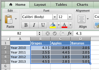
Format Number Options for Chart Data Labels in Excel 2011 for Mac
Quick Tip: Excel 2013 offers flexible data labels - TechRepublic
Post a Comment for "39 how to format data labels in excel charts"