38 excel data labels from third column
How to Add Labels to Scatterplot Points in Excel - Statology Next, click anywhere on the chart until a green plus (+) sign appears in the top right corner. Then click Data Labels, then click More Options… In the Format Data Labels window that appears on the right of the screen, uncheck the box next to Y Value and check the box next to Value From Cells. Excel, giving data labels to only the top/bottom X% values 1) Create a data set next to your original series column with only the values you want labels for (again, this can be formula driven to only select the top / bottom n values). See column D below. 2) Add this data series to the chart and show the data labels. 3) Set the line color to No Line, so that it does not appear! 4) Volia! See Below! Share
How to Print Labels From Excel - EDUCBA Navigate towards the folder where the excel file is stored in the Select Data Source pop-up window. Select the file in which the labels are stored and click Open. A new pop up box named Confirm Data Source will appear. Click on OK to let the system know that you want to use the data source. Again a pop-up window named Select Table will appear.

Excel data labels from third column
Data labels not displayed correctly - Excel Help Forum The data label is a date value that selects values from the date column. The Primary axis is categorized based on 2 values. The secondary axis is Month. The data labels are displayed accurately as per the month except the 3 labels. The first series is the difference between F and E.The second series is the difference between the J and K column. Custom data labels in a chart - Get Digital Help Add data labels Press with right mouse button on on a column Press with left mouse button on "Add Data Labels" Double press with left mouse button on a data label Deselect Value Select Category name Press with left mouse button on Close Get the Excel file Custom-data-labels-in-a-chartv3.xlsx Charts category Add pictures to a chart axis How to add data labels from different columns in an Excel chart? Step 5 To add data labels, right-click the set of data in the chart, then pick the Add Data Labels option in Add Data Labels from the context menu. This will bring up a new window. Step 6 This is the data label that is currently shown in the chart. Step 7 If you click any data label, then all data labels will be selected.
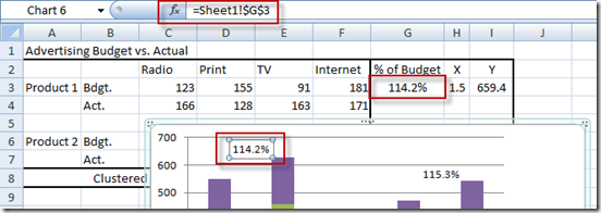
Excel data labels from third column. Custom Data Labels with Colors and Symbols in Excel Charts - [How To ... The way I know is to simply click the data label once and clicking it again will select the particular data label which you can then format with desired color. And of course you will have to do it for each data label separately. Tiring right? And above that it is "hard" coloring the labels. How to Change Excel Chart Data Labels to Custom Values? - Chandoo.org First add data labels to the chart (Layout Ribbon > Data Labels) Define the new data label values in a bunch of cells, like this: Now, click on any data label. This will select "all" data labels. Now click once again. At this point excel will select only one data label. Go to Formula bar, press = and point to the cell where the data label ... Custom Excel Chart Label Positions • My Online Training Hub Custom Excel Chart Label Positions - Setup. The source data table has an extra column for the 'Label' which calculates the maximum of the Actual and Target: The formatting of the Label series is set to 'No fill' and 'No line' making it invisible in the chart, hence the name 'ghost series': The Label Series uses the 'Value ... How to Use Cell Values for Excel Chart Labels - How-To Geek Select the chart, choose the "Chart Elements" option, click the "Data Labels" arrow, and then "More Options." Uncheck the "Value" box and check the "Value From Cells" box. Select cells C2:C6 to use for the data label range and then click the "OK" button. The values from these cells are now used for the chart data labels.
Prevent Overlapping Data Labels in Excel Charts - Peltier Tech Overlapping Data Labels. Data labels are terribly tedious to apply to slope charts, since these labels have to be positioned to the left of the first point and to the right of the last point of each series. This means the labels have to be tediously selected one by one, even to apply "standard" alignments. Apply Custom Data Labels to Charted Points - Peltier Tech Click once on a label to select the series of labels. Click again on a label to select just that specific label. Double click on the label to highlight the text of the label, or just click once to insert the cursor into the existing text. Type the text you want to display in the label, and press the Enter key. Mac Excel 2008 - How to add Data Labels for Scatter Plot coming from ... In Excel 2008, to select X axis for the labels: go to 'Formatting palette' navigate to 'Chart Option' Under 'Other options' select "category name' in Labels. A AsherS New Member Joined Feb 9, 2012 Messages 9 Jul 30, 2014 #3 Cyrilbrd, this does not add a label from another column. This only displays the X-value and does not solve the issue. cyrilbrd Adding rich data labels to charts in Excel 2013 | Microsoft 365 Blog Putting a data label into a shape can add another type of visual emphasis. To add a data label in a shape, select the data point of interest, then right-click it to pull up the context menu. Click Add Data Label, then click Add Data Callout . The result is that your data label will appear in a graphical callout.
How can I add data labels from a third column to a scatterplot? Do you want to add data labels to the 3rd column values in the chart? Highlight the 3rd column range in the chart. Click the chart, and then click the Chart Layout tab. Under Labels, click Data Labels, and then in the upper part of the list, click the data label type that you want. VLOOKUP Hack #4: Column Labels - Excel University The 3rd argument of the VLOOKUP function is officially known as col_index_num. This represents the position of the value you want returned. For example, if you want to return the amount from the 2nd position, or column, within the lookup range, you would enter 2 for the argument. Consider the screenshot below. Using Data Labels from a Third Data Column in an Chart Excel 2013, allows you to select Data Labels locations from a Dialog box Prior to that it had to be done either manually or via a Macro To do it manually Select a Series Add a Data Label Select the Data Labels Then select an Individual Data Label In the formula bar =$D$2 (Cell reference to your new labels) Repeat for all Labels G guna_sekar87 How to Print Labels from Excel Using Database Connections - TEKLYNX How to Print Labels from Excel Using TEKLYNX Label Design Software: Open label design software. Click on Data Sources, and then click Create/Edit Query. Select Excel and name your database. Browse and attach your database file. Save your query so it can be used again in the future. Select the necessary fields (columns) that you would like to ...
Bubble Chart: How to create it in excel - DataWitzz
Create a multi-level category chart in Excel - ExtendOffice 1.3) In the third column, type in each data for the subcategories. 2. Select the data range, click Insert > Insert Column or Bar Chart > Clustered Bar. 3. Drag the chart border to enlarge the chart area. See the below demo. 4. Right click the bar and select Format Data Series from the right-clicking menu to open the Format Data Series pane.
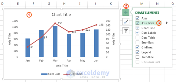
Excel Chart Elements: Parts of Charts in Excel | ExcelDemy
Show third column as label in graph | MrExcel Message Board I have a data set consisting of three columns. Column A is a name, B is an x-axis value, and C is an y-axis value. I use the B and C column to plot the positions in an X/Y point diagram. This is working nicely. But is there a way for me to get the value in the A column as the label for the...

excel vba - VBA Change Data Labels on a Stacked Column chart from 'Value' to 'Series name ...
Can I add data labels from an unrelated column to a simple 2-D column ... I would like to add data labels to the vertical chart representations with values from a third column. I am trying to show how many input/data points were included for each displayed column percentage (height) on the chart. The third column values range from 10-200, with an couple outliers up to 5,500, so a third axis doesn't display the data well.

31 How To Label Excel Columns - Labels For Your Ideas
Change the format of data labels in a chart To get there, after adding your data labels, select the data label to format, and then click Chart Elements > Data Labels > More Options. To go to the appropriate area, click one of the four icons ( Fill & Line, Effects, Size & Properties ( Layout & Properties in Outlook or Word), or Label Options) shown here.

How to Create Multi-Category Chart in Excel - Excel Board
How to add data labels from different column in an Excel chart? This method will guide you to manually add a data label from a cell of different column at a time in an Excel chart. 1. Right click the data series in the chart, and select Add Data Labels > Add Data Labels from the context menu to add data labels. 2.
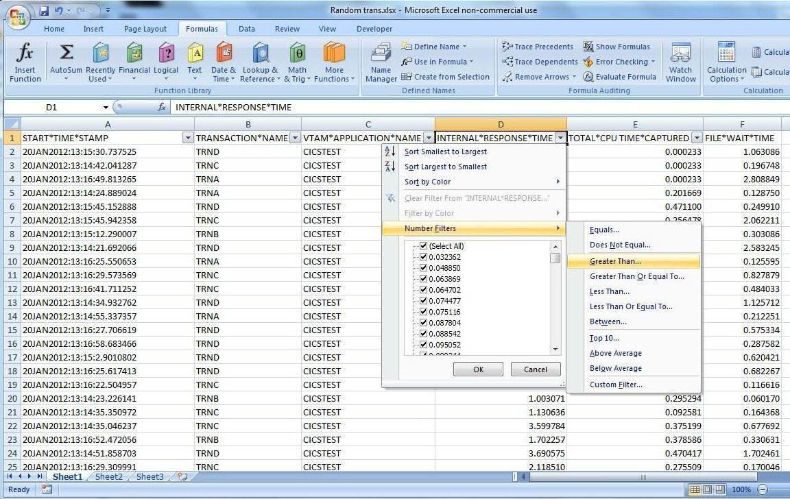
Analyze MXG mainframe performance data with Excel
Adding Data Labels To An Excel Chart | MyExcelOnline In our example below, I add a Data Label to a column chart and then I format the data label using CTRL+1. I then select to custom format the numbers so it shows the values as thousands by adding a comma , after each zero and then showing the work k by adding "k". Example Custom Number Format: [$$-1004]#,##0 ,"k" ;- [$$-1004]#,##0 ,"k".

How to count unique column data in an excel sheet - Stack Overflow
Add or remove data labels in a chart - support.microsoft.com Right-click the data series or data label to display more data for, and then click Format Data Labels. Click Label Options and under Label Contains, select the Values From Cells checkbox. When the Data Label Range dialog box appears, go back to the spreadsheet and select the range for which you want the cell values to display as data labels.

How to Create Multi-Category Chart in Excel - Excel Board
Add Custom Labels to x-y Scatter plot in Excel Step 1: Select the Data, INSERT -> Recommended Charts -> Scatter chart (3 rd chart will be scatter chart) Let the plotted scatter chart be. Step 2: Click the + symbol and add data labels by clicking it as shown below. Step 3: Now we need to add the flavor names to the label. Now right click on the label and click format data labels.
How-to Add Centered Labels Above an Excel Clustered Stacked Column Chart - Excel Dashboard Templates
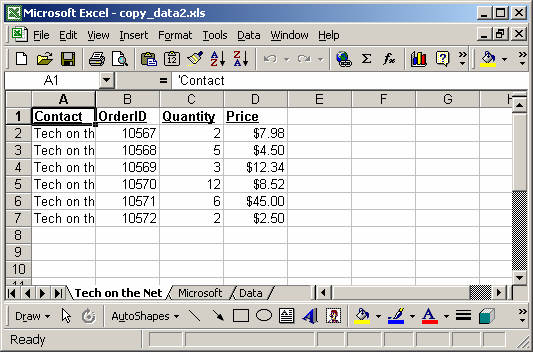
How to Create Labels in Word from an Excel Spreadsheet - Online Tech Tips In the File Explorer window that opens, navigate to the folder containing the Excel spreadsheet you created above. Double-click the spreadsheet to import it into your Word document. Word will open a Select Table window. Here, select the sheet that contains the label data. Tick mark the First row of data contains column headers option and select OK.
MS Excel 2003: Test each value in column A and copy matching values into new sheets
How to create Custom Data Labels in Excel Charts - Efficiency 365 To customize it, click on the arrow next to Data Labels and choose More Options … Unselect the Value option and select the Value from Cells option. Choose the third column (without the heading) as the range. Now we have exactly what we want. Some labels may overlap the chart elements and they have a transparent background by default.

Getting Started > Getting Started with XY Plots > Getting Started with XY Plots - Data From ...
How to add data labels from different columns in an Excel chart? Step 5 To add data labels, right-click the set of data in the chart, then pick the Add Data Labels option in Add Data Labels from the context menu. This will bring up a new window. Step 6 This is the data label that is currently shown in the chart. Step 7 If you click any data label, then all data labels will be selected.

How to add data labels from different column in an Excel chart?
Custom data labels in a chart - Get Digital Help Add data labels Press with right mouse button on on a column Press with left mouse button on "Add Data Labels" Double press with left mouse button on a data label Deselect Value Select Category name Press with left mouse button on Close Get the Excel file Custom-data-labels-in-a-chartv3.xlsx Charts category Add pictures to a chart axis

Print Only Selected Data In Excel : We can select those specific cells as the print area ...
Data labels not displayed correctly - Excel Help Forum The data label is a date value that selects values from the date column. The Primary axis is categorized based on 2 values. The secondary axis is Month. The data labels are displayed accurately as per the month except the 3 labels. The first series is the difference between F and E.The second series is the difference between the J and K column.
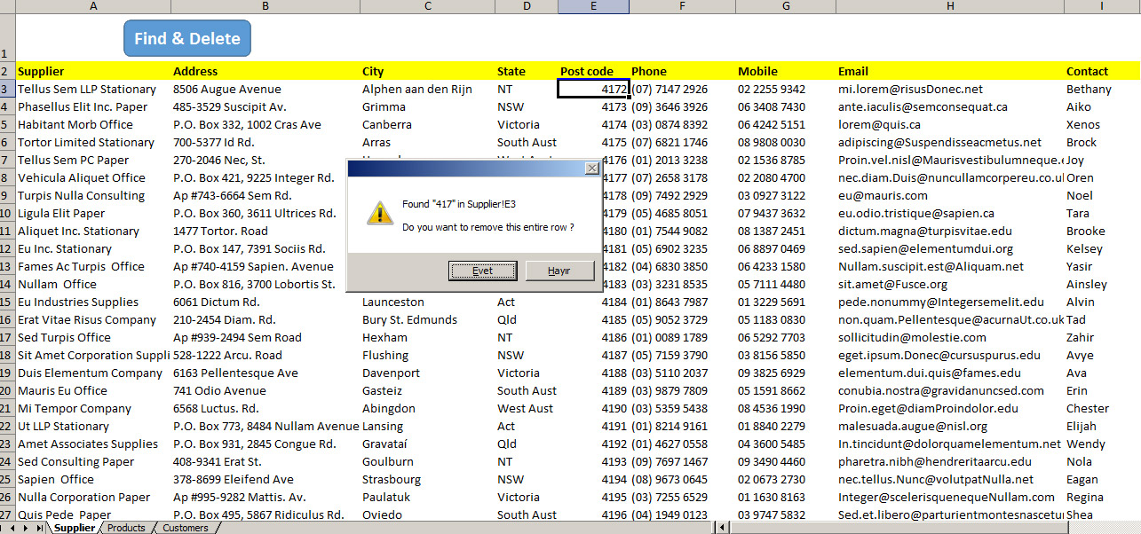
Excel Vba Find And Delete - Hints And Tips About Technology ,Computer And Life
How to Add Data Labels on Chart Column in Excel 2007 VID#11 - YouTube

Merge Data from an Excel Workbook into a Word Document
Post a Comment for "38 excel data labels from third column"