41 how to change excel chart data labels to custom values

Use custom formats in an Excel chart's axis and data labels Right-click the Axis area and choose Format Axis from the context menu. If you don't see Format Axis, right-click another spot. Choose Number in the left pane. (In Excel 2003, click the Number ... Is there a way to change the order of Data Labels? Please try to double click the the part of the label value, and choose the one you want to show to change the order. Thanks, Rena ----------------------- * Beware of scammers posting fake support numbers here. * Once complete conversation about this topic, kindly Mark and Vote any replies to benefit others reading this thread. Report abuse

Change axis labels in a chart - support.microsoft.com Right-click the category labels you want to change, and click Select Data. In the Horizontal (Category) Axis Labels box, click Edit. In the Axis label range box, enter the labels you want to use, separated by commas. For example, type Quarter 1,Quarter 2,Quarter 3,Quarter 4. Change the format of text and numbers in labels

How to change excel chart data labels to custom values

Apply Custom Data Labels to Charted Points - Peltier Tech Click once on a label to select the series of labels. Click again on a label to select just that specific label. Double click on the label to highlight the text of the label, or just click once to insert the cursor into the existing text. Type the text you want to display in the label, and press the Enter key. How to Change Axis Values in Excel - Excelchat To change x axis values to "Store" we should follow several steps: Right-click on the graph and choose Select Data: Figure 2. Select Data on the chart to change axis values. Select the Edit button and in the Axis label range select the range in the Store column: Figure 3. Change horizontal axis values. How to add and customize chart data labels - Get Digital Help Double press with left mouse button on with left mouse button on a data label series to open the settings pane. Go to tab "Label Options" see image to the right. You have here the option to change the data label position relative to the data point. Center - This places the data label right on the data point.

How to change excel chart data labels to custom values. How to add or move data labels in Excel chart? - ExtendOffice 1. Click the chart to show the Chart Elements button . 2. Then click the Chart Elements, and check Data Labels, then you can click the arrow to choose an option about the data labels in the sub menu. See screenshot: How to create Custom Data Labels in Excel Charts Two ways to do it. Click on the Plus sign next to the chart and choose the Data Labels option. We do NOT want the data to be shown. To customize it, click on the arrow next to Data Labels and choose More Options … Unselect the Value option and select the Value from Cells option. Choose the third column (without the heading) as the range. Add or remove data labels in a chart - support.microsoft.com Click Label Options and under Label Contains, pick the options you want. Use cell values as data labels You can use cell values as data labels for your chart. Right-click the data series or data label to display more data for, and then click Format Data Labels. Click Label Options and under Label Contains, select the Values From Cells checkbox. How to Customize Your Excel Pivot Chart Data Labels - dummies If you want to label data markers with a category name, select the Category Name check box. To label the data markers with the underlying value, select the Value check box. In Excel 2007 and Excel 2010, the Data Labels command appears on the Layout tab. Also, the More Data Labels Options command displays a dialog box rather than a pane.

Edit titles or data labels in a chart - support.microsoft.com The first click selects the data labels for the whole data series, and the second click selects the individual data label. Right-click the data label, and then click Format Data Label or Format Data Labels. Click Label Options if it's not selected, and then select the Reset Label Text check box. Top of Page How to add data labels from different column in an Excel chart? Click any data label to select all data labels, and then click the specified data label to select it only in the chart. 3. Go to the formula bar, type =, select the corresponding cell in the different column, and press the Enter key. See screenshot: 4. Repeat the above 2 - 3 steps to add data labels from the different column for other data points. Custom Excel Chart Label Positions - YouTube Customize Excel Chart Label Positions with a ghost/dummy series in your chart. Download the Excel file and see step by step written instructions here: https:... Excel charts: add title, customize chart axis, legend and data labels ... Select the chart and go to the Chart Tools tabs ( Design and Format) on the Excel ribbon. Right-click the chart element you would like to customize, and choose the corresponding item from the context menu. Use the chart customization buttons that appear in the top right corner of your Excel graph when you click on it.

How to change chart axis labels' font color and size in Excel? 1. Right click the axis where you will change all negative labels' font color, and select the Format Axis from the right-clicking menu. 2. Do one of below processes based on your Microsoft Excel version: (1) In Excel 2013's Format Axis pane, expand the Number group on the Axis Options tab, click the Category box and select Number from drop down ... Using the CONCAT function to create custom data labels for an Excel chart Use the chart skittle (the "+" sign to the right of the chart) to select Data Labels and select More Options to display the Data Labels task pane. Check the Value From Cells checkbox and select the cells containing the custom labels, cells C5 to C16 in this example. Adding rich data labels to charts in Excel 2013 - Microsoft 365 Blog Putting a data label into a shape can add another type of visual emphasis. To add a data label in a shape, select the data point of interest, then right-click it to pull up the context menu. Click Add Data Label, then click Add Data Callout . The result is that your data label will appear in a graphical callout. excel - How do I update the data label of a chart? - Stack Overflow Select the data label Then, place your cursor in Excel's Formula Bar, and enter the formula like ='Sheet2'!$C$3. Now, that data label is associated by the formula, to the cell C3, which contains the desired data label that we built above. Repeat as needed. Note: The sheet name is required in this formula.

Moving X-axis labels at the bottom of the chart below negative values in Excel - PakAccountants.com

Custom Data Labels with Colors and Symbols in Excel Charts - [How To] To apply custom format on data labels inside charts via custom number formatting, the data labels must be based on values. You have several options like series name, value from cells, category name. But it has to be values otherwise colors won't appear. Symbols issue is quite beyond me.

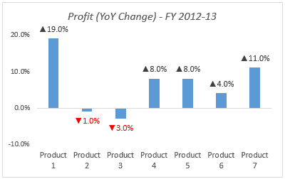
Color Negative Chart Data Labels in Red with downward arrow

How to Change Excel Chart Data Labels to Custom Values? First add data labels to the chart (Layout Ribbon > Data Labels) Define the new data label values in a bunch of cells, like this: Now, click on any data label. This will select "all" data labels. Now click once again. At this point excel will select only one data label.

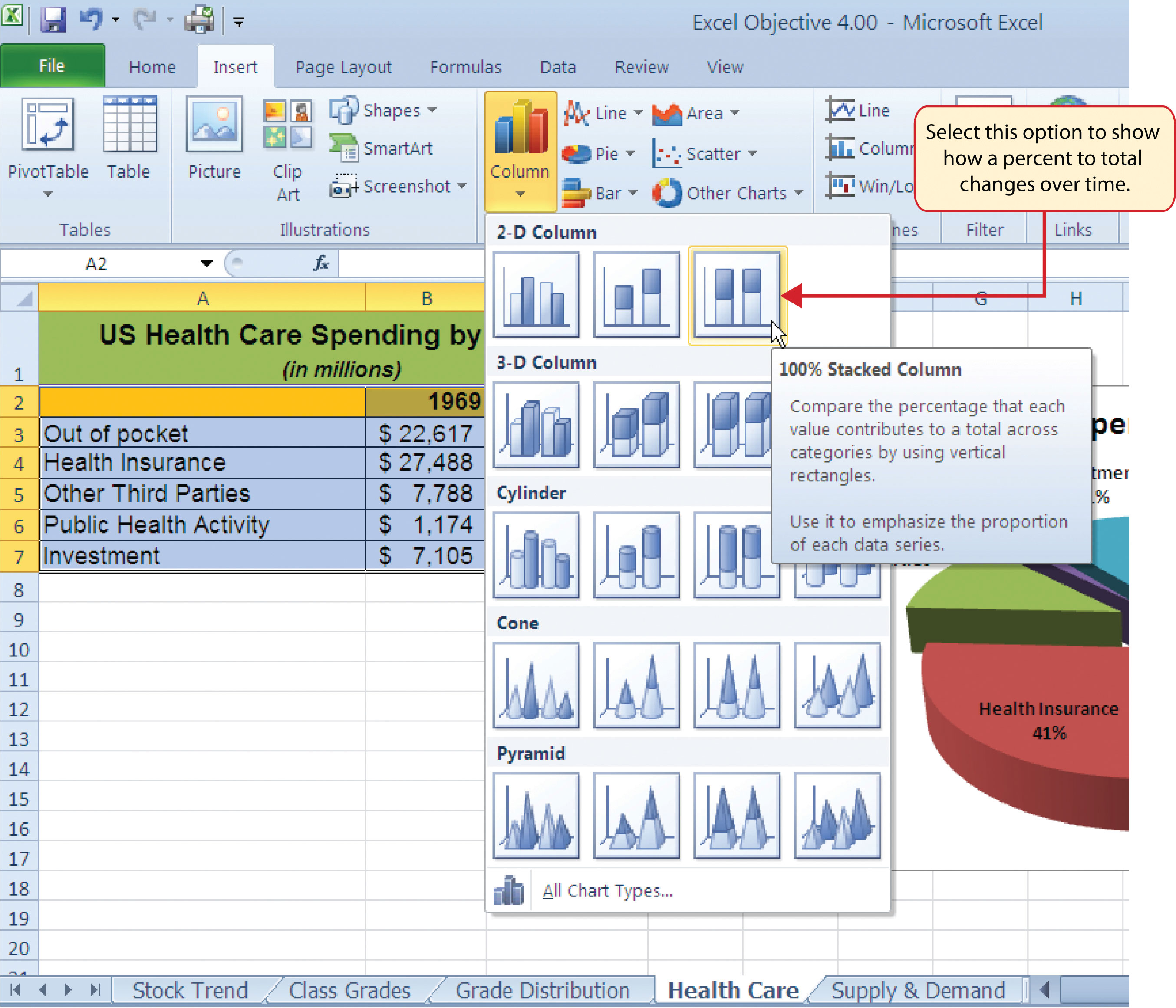
How to Make a Pie Chart in Excel & Add Rich Data Labels to The Chart!

Change the format of data labels in a chart To get there, after adding your data labels, select the data label to format, and then click Chart Elements > Data Labels > More Options. To go to the appropriate area, click one of the four icons ( Fill & Line, Effects, Size & Properties ( Layout & Properties in Outlook or Word), or Label Options) shown here.

How to Create a Timeline Chart in Excel - Automate Excel

Custom data labels in a chart - Get Digital Help Press with right mouse button on on any data series displayed in the chart. Press with mouse on "Add Data Labels". Press with mouse on Add Data Labels". Double press with left mouse button on any data label to expand the "Format Data Series" pane. Enable checkbox "Value from cells".

Custom data labels in a chart | Get Digital Help - Microsoft Excel resource

How to Use Cell Values for Excel Chart Labels - How-To Geek Select the chart, choose the "Chart Elements" option, click the "Data Labels" arrow, and then "More Options." Uncheck the "Value" box and check the "Value From Cells" box. Select cells C2:C6 to use for the data label range and then click the "OK" button. The values from these cells are now used for the chart data labels.

Excel charts: add title, customize chart axis, legend and data labels

Format Data Labels in Excel- Instructions - TeachUcomp, Inc. To format data labels in Excel, choose the set of data labels to format. To do this, click the "Format" tab within the "Chart Tools" contextual tab in the Ribbon. Then select the data labels to format from the "Chart Elements" drop-down in the "Current Selection" button group. Then click the "Format Selection" button that ...

30 Definition Of Label In Excel - Labels Information List

Change the data series in a chart - support.microsoft.com Click anywhere in your chart. Click the Chart Filters button next to the chart. On the Values tab, check or uncheck the series or categories you want to show or hide. Click Apply. If you want to edit or rearrange the data in your series, click Select Data, and then follow steps 2-4 in the next section.

Create a column chart with percentage change in Excel

Custom Chart Data Labels In Excel With Formulas Follow the steps below to create the custom data labels. Select the chart label you want to change. In the formula-bar hit = (equals), select the cell reference containing your chart label's data. In this case, the first label is in cell E2. Finally, repeat for all your chart laebls.

Share :